永井 忠一 2023.8.20
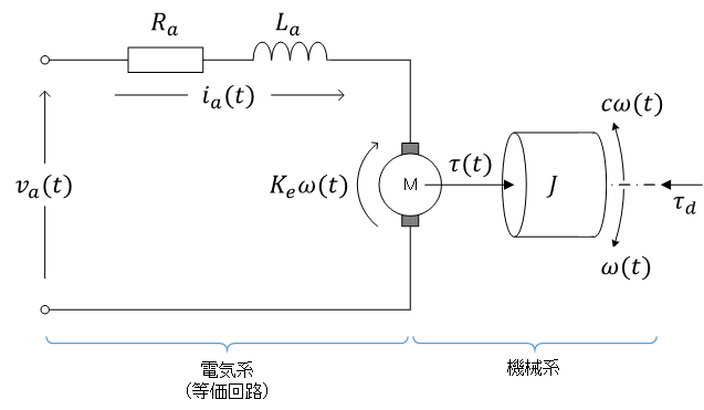
等価回路(以前のページの図を描き直し)
(図で、\( \tau_d \) は外乱トルク)
| 電気的性質 | 機械的性質 |
|---|---|
|
|
|
|
電流 \( i_a \) に比例したトルク \( K_t i_a \) が発生する。と同時に、回転角速度 \( \omega \) に比例した逆起電力 \( K_e\omega \) が発生する(同時に、発電機でもある)
\[ \left\{ \begin{align} &v_a = R_a i_a + L_a s i_a + K_e\omega \\ &\tau = K_t i_a \\ &\tau = Js\omega + c\omega + \tau_d \end{align} \right. \]
(\( s \) は、ラプラス変換の微分演算子)
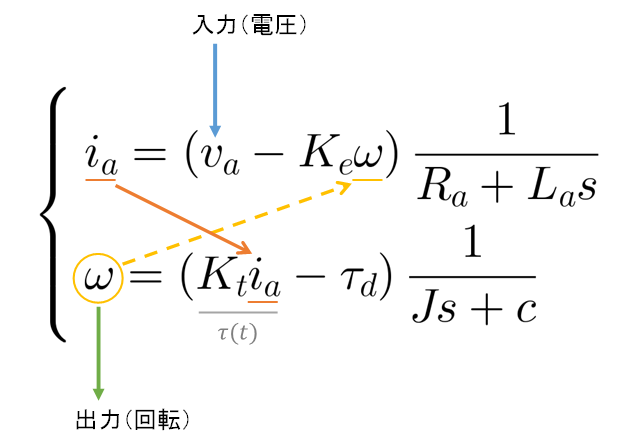
連立方程式を式変形
| \[ \begin{align} v_a &= R_a i_a + L_a s i_a + K_e\omega \\ v_a - K_e\omega &= (R_a + L_a s)i_a \\ i_a &= \frac{v_a - K_e\omega}{R_a + L_a s} \end{align} \] | \[ \left\{ \begin{align} &i_a = \frac{v_a - K_e\omega}{R_a + L_a s} \\ &\omega = \frac{K_t i_a - \tau_d}{Js + c} \end{align} \right. \] |
| \[ \begin{align} \tau &= Js\omega + c\omega + \tau_d \\ \tau - \tau_d &= (Js + c)\omega \\ \omega &= \frac{\tau - \tau_d}{Js + c} \\ \omega &= \frac{K_t i_a - \tau_d}{Js + c} \end{align} \] |
DC motor の連立方程式 \( \boxed{ \left\{ \begin{align} \text{電気系} \\ \text{機械系} \end{align} \right. } \) の意味の理解(モータの機能と、発電機としての機能とが同時に働いている)
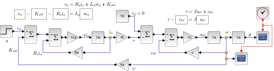
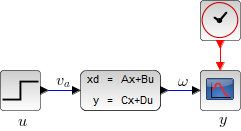
DC motor の伝達関数表現。Xcos を利用
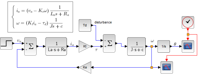
(\( 1/s \) は積分。角速度を積分して角度 \( \theta \) 。図右端の『\( \omega\rightarrow\boxed{\frac{1}{s}}\rightarrow\theta \)』)
(Xcos のプログラム)
伝達関数から → 状態方程式を求める(実現、実現問題)
伝達関数のブロック線図を分解
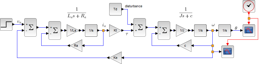
(Xcos のプログラム)
ブロック線図の伝達関数の変形の確認。フィードバック接続 \( \boxed{ \frac{1}{L_a s + R_a} } \) を検算
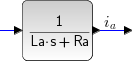 | ⇔ | 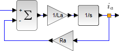 |
(\( R_a \)、\( L_a \) は適当に与えている)
| Scilab | Octave |
|---|---|
|
|
(Scilab では、フィードバック接続に「/.」演算子を使用する。Octave では、control パッケージにある feedback() 関数を使う)
ブロック線図と式の対応とを確認
式 再掲載\[ \left\{ \begin{align} &v_a = R_a i_a + L_a s i_a + K_e\omega \\ &\tau = K_t i_a \\ &\tau = Js\omega + c\omega + \tau_d \end{align} \right. \](第1式と第3式を式変形(移項)している。また、外乱項は無いものとしている)
(Xcos のプログラム)
伝達関数のブロック線図から状態方程式と出力方程式を求める
ブロック線図に必要な情報をすべて記入(外乱の項は省略)
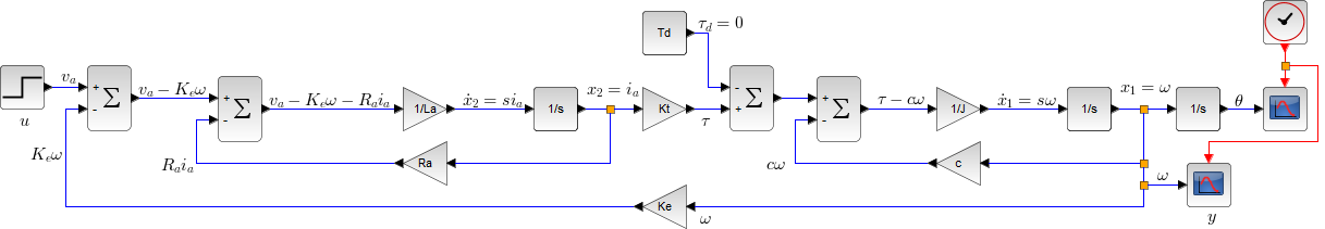
(Xcos のプログラム)
ブロック線図から式を作成。\( \dot x_1 \) について方程式を立てる:\[ \begin{align} \dot x_1 &= \frac{1}{J}\left(\tau - c x_1\right) \\ &= \frac{1}{J}\left(K_t x_2 - c x_1\right) \\ &= -\frac{c}{J}x_1 + \frac{K_t}{J}x_2 \end{align} \]同様に、\( \dot x_2 \) についての方程式:\[ \begin{align} \dot x_2 &= \frac{1}{L_a}\left(u - K_e x_1 - R_a x_2\right) \\ &= -\frac{K_e}{L_a}x_1 - \frac{R_a}{L_a}x_2 + \frac{1}{L_a}u \end{align} \]
得られた連立方程式\[ \left\{ \begin{align} &\dot x_1 = -\frac{c}{J}x_1 + \frac{K_t}{J}x_2 \\ &\dot x_2 = -\frac{K_e}{L_a}x_1 - \frac{R_a}{L_a}x_2 + \frac{1}{L_a}u \end{align} \right. \]を行列の形で式を整理する
∴ DC motor の状態方程式\[ \begin{align} \dot{\vec x} &= \begin{bmatrix}\dot x_1 \\ \dot x_2\end{bmatrix} = \begin{bmatrix}-\frac{c}{J} & \frac{K_t}{J} \\ -\frac{K_e}{L_a} & -\frac{R_a}{L_a}\end{bmatrix}\begin{bmatrix}x_1 \\ x_2\end{bmatrix} + \begin{bmatrix}0 \\ \frac{1}{L_a}\end{bmatrix}u \\ &= \begin{bmatrix}\dot \omega \\ \dot{i_a}\end{bmatrix} = \begin{bmatrix}-\frac{c}{J} & \frac{K_t}{J} \\ -\frac{K_e}{L_a} & -\frac{R_a}{L_a}\end{bmatrix}\begin{bmatrix}\omega \\ i_a\end{bmatrix} + \begin{bmatrix}0 \\ \frac{1}{L_a}\end{bmatrix}v_a \end{align} \]出力方程式\[ \begin{align} y &= \omega = \begin{bmatrix}1 & 0\end{bmatrix}\begin{bmatrix}x_1 \\ x_2\end{bmatrix} \\ &= \omega = \begin{bmatrix}1 & 0\end{bmatrix}\begin{bmatrix}\omega \\ i_a\end{bmatrix} \end{align} \](電流 \( i_a \) は観測できない場合)
まとめて、状態空間表現\[ \left\{ \begin{align} &\dot{\vec x} = A\vec x + B\vec u \\ &y = C\vec x + D\vec u \end{align}\right. \]は(直達項は無い「\( D = 0 \)」として)\[ \left\{ \begin{align} &\dot{\vec x} = \begin{bmatrix}-\frac{c}{J} & \frac{K_t}{J} \\ -\frac{K_e}{L_a} & -\frac{R_a}{L_a}\end{bmatrix}\vec x + \begin{bmatrix}0 \\ \frac{1}{L_a}\end{bmatrix}u \\ &y = \begin{bmatrix}1 & 0\end{bmatrix}\vec x \end{align}\right. \]となる
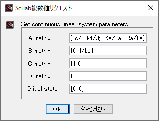
入力と出力、それから状態変数ベクトルが時間の関数であることを強調して書けば\[ \left\{ \begin{align} &\dot{\vec x}(t) = \begin{bmatrix}-\frac{c}{J} & \frac{K_t}{J} \\ -\frac{K_e}{L_a} & -\frac{R_a}{L_a}\end{bmatrix}\vec x(t) + \begin{bmatrix}0 \\ \frac{1}{L_a}\end{bmatrix}u(t) \\ &y(t) = \begin{bmatrix}1 & 0\end{bmatrix}\vec x(t) \end{align}\right. \](また、\( A \) 行列、\( B \) 行列、\( C \) 行列(、\( D \) 行列)は、定数行列。時不変システム)
(Xcos の CLSS ブロックを利用)
 |
 |
(Xcos のプログラム)
例(マブチモーター RE-140RA-2270)
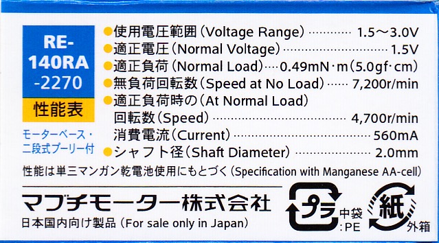
(Webにあるものと、なぜか諸元が違っている)
| MODEL | VOLTAGE | NO LOAD | AT MAXIMUM EFFICIENCY | STALL | ||||||||
|---|---|---|---|---|---|---|---|---|---|---|---|---|
| OPERATING RANGE | NOMINAL | SPEED | CURRENT | SPEED | CURRENT | TORQUE | OUTPUT | TORQUE | CURRENT | |||
| r/min | A | r/min | A | mN·m | g·cm | W | mN·m | g·cm | A | |||
| RE-140RA-2270 | 1.5〜3.0 | 1.5V CONSTANT | 8100 | 0.21 | 6150 | 0.66 | 0.66 | 6.7 | 0.42 | 2.74 | 28 | 2.10 |
基本特性。トルクと回転速度(角速度)
| Maxima | Python |
|---|---|
|
|
(諸元の値が違っているので、数字を読みかえて計算)
(変数名の rated_ は、定格の意味)
∴ stall torque ≈ 2.74 [mN·m]
(stall torqueは、起動トルクとも呼ばれる)
トルクと電流
| Python |
|---|
|
| Maxima |
|
∴ stall current ≈ 2.1 [A]
定格トルクの点を、0.49 mN·m として換算(諸元がはっきりしないので)
| Python |
|---|
|
T-N線図

作図プログラム
| Python |
|---|
|
トルク定数 \( K_\mathrm T \)、逆起電力定数 \( K_\mathrm E \)
| Maxima | Python |
|---|---|
| |
(トルク ∝ 電流)
(理想DC motorでは、\( K_\mathrm T = K_\mathrm E \) となる)
(\( K_\mathrm E \) の単位 \( [\mathrm V/(\mathrm{rad}/\mathrm s)] = [\mathrm{Vs}/\mathrm{rad}] = [\mathrm{Wb}/\mathrm{rad}] \)。\( \mathrm{Wb} \) は磁束の単位で、\( \mathrm{Wb}/\mathrm{rad} \) は「1 rad あたりの磁束」という意味)
印加電圧 \( V \) の変化。DC motorの式を\[ \left\{ \begin{align} & \tau = K_\mathrm T I \\ & E = K_\mathrm E\omega\\ & V = RI + E \end{align} \right. \]\( \omega \) について解く
| Maxima |
|---|
|
得られた、1次式\[ \omega = -\frac{R}{K_\mathrm E K_\mathrm T}\tau + \frac{V}{K_\mathrm E} \]
1.5〜3.0 V の場合

作図プログラム
| Python | Maxima |
|---|---|
|
|
| R | |
|
Powerと損失

(Lossは、ほとんどが発熱となる)
作図プログラム
| Python |
|---|
|
© 2023, 2025 Tadakazu Nagai